Trade Network Updates, Part 1

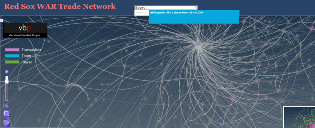
A few years back (2016 o be specific) I created network graphs displaying the history of trades made for each MLB franchise, using transactions data from the wonderful Retrosheet project. These graphs presented more than a few challenges in how to present the data but I wound up with what I consider to be a very interesting set of results, which you can find here. I also created some posts on the process at that time, found here and here.

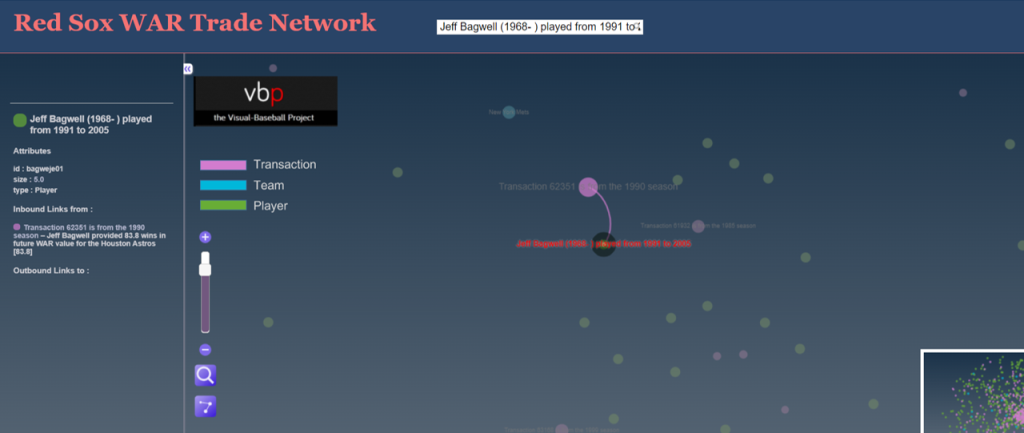
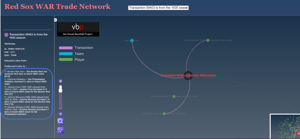
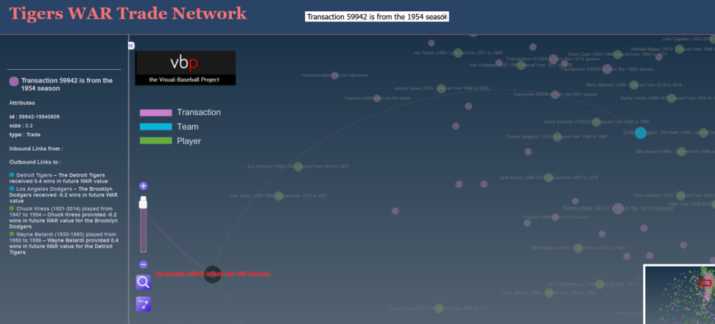
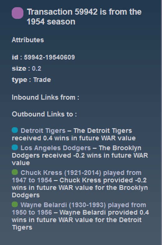
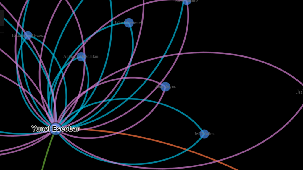
Here’s a snapshot within a graph:

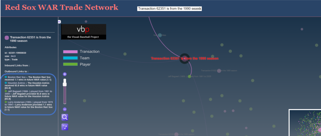
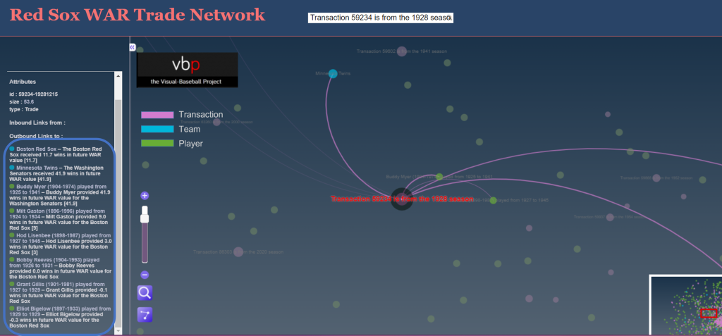
Six seasons have elapsed since I created those graphs, so I thought it was beyond time to update them, but this time with a twist. Last fall I came across a great dataset that captures an array of advanced sabermetric statistics which I hope to use on a regular basis. These statistics can be used to assess a player’s true value relative to his peers each season. What if I could incorporate those into the trade network updates to show the post-trade value of each player to their new team? Ideally, this will help to show the value of each trade and which team wound up getting the better part of the deal.

Of course this would involve adding a degree of complexity to the MySQL code for pulling the data and shaping it for use in creating network graphs. However, the end result could be very revealing and worthwhile. Today I’m at the start of the process, tinkering with SQL code to extract the data in a proper format. Here’s an example:

SELECT h.player_name, p.playerID, tr.season, tr.TransactionID, tr.TeamFrom, tr.TeamTo, ROUND(SUM(h.WAR162),1) as WAR

FROM historical_WAR_and_more h
INNER JOIN People p
ON h.key_bbref = p.bbrefID
INNER JOIN trades2021 tr
ON p.retroID = tr.Player

WHERE tr.season >= 1901 and h.year_ID > tr.season and h.team_ID = tr.TeamTo AND tr.Type = ‘T’

GROUP BY h.player_name, p.playerID, tr.season, tr.TransactionID, tr.TeamFrom, tr.TeamTo

In this case, I’m looking at the cumulative WAR (Wins Above Replacement) for each traded player with their new team. This could be a single season total or the sum of many years in some cases. Here are some results:

We now have post-trade results (starting if the season following the trade) as measured by WAR for each traded player. We see one fairly substantial figure – the second Aaron Harang trade which netted 16.9 WAR points for his new team, the Cincinnati Reds (CIN in the results). Given that a single season WAR above 3 or 4 is considered substantial, it’s clear that his new team probably benefited from a few of those high-value seasons. What we can’t see yet is what they gave away in their half of the trade.

Fortunately, we can access this using the TransactionID field, which provides all the information for each party within the trade. But we’ll save that for another day as I figure out the next progression of the code. As always, thanks for reading!

FacebooktwitterlinkedinrssFacebooktwitterlinkedinrssby feather
FacebooktwitterredditpinterestlinkedinmailFacebooktwitterredditpinterestlinkedinmailby feather

Major League Baseball Trade Networks, Part 2

Welcome to Part 2 in our miniseries on building baseball (MLB) trade networks with Gephi. In the first post, the focus was on procuring and preparing the data using MySQL. The goal was to create nodes and edges that could be easily imported to Gephi. Gephi does allow for some data manipulation post-import, but I’ve learned from experience to do the main parts of the job with either SQL code or within spreadsheet software like Excel or Calc.

With our data readied for import, we’ll now move on to the more fun parts of the process, where we get to visualize the data and see any underlying patterns. Gephi is an ideal tool for this, as it allows us to try out many different algorithms, especially in version 0.8.2. The newer 0.9 versions are faster, but have not fully caught up on the plugin side at this writing, so options are a bit more limited. One other caveat – I frequently run into Java issues when using Gephi, so save your work often and be prepared to shut down and restart Gephi periodically.

We’ll kick off this part of the process by importing the data, nodes first, followed by edges. The reason I prefer this order is that nodes will be automatically created if we start with the edge file import, and they won’t contain any extra fields you may have added using your database or spreadsheet processes.

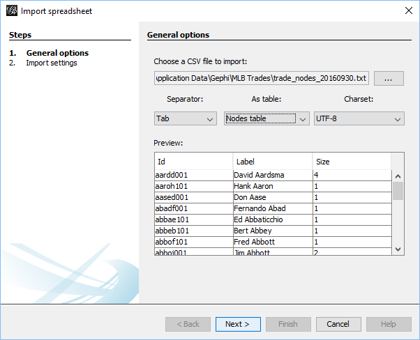
Here’s the node import window, showing the appropriate file input:

Gephi node import window

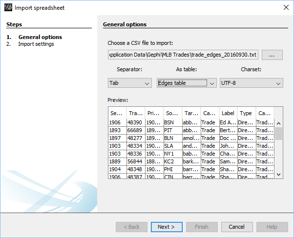
Once the node import process is complete, we turn to the edges file, and follow a similar sequence of steps. Here’s our starting point:

Gephi edge import window

After the data has been imported, it’s time to move to the Overview tab, where we’ll see a dense mess of nodes and edges, especially if we have a fair sized dataset. Something like this:

Impossibly dense hairball network

Gephi offers a variety of interesting algorithms, each more or less appropriate based on the underlying dataset. In our case, the dataset is of a moderate size, with more than 8,000 nodes and nearly 62,000 edges. This immediately rules out the use of simple layouts such as the circular algorithms, as it would prove immensely challenging to display, even when we take it to an interactive output. At the other end of the sophistication level lie the force-directed layouts, which apply a significant dose of science and math within their respective algorithms. In Gephi, the Force Atlas 2 is quite popular, but it tends to run very slowly unless coupled with enormous levels of RAM. So where to go with our choice for this data?

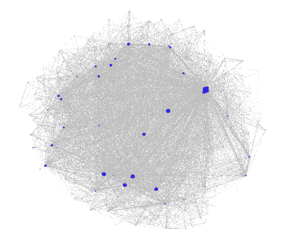
I elected to take a two step approach, using the extremely fast (if less precise) OpenOrd algorithm for the original data. This provides a nice view of the network within a few minutes, making it a good starting point for our next steps.

Trade network with OpenOrd layout

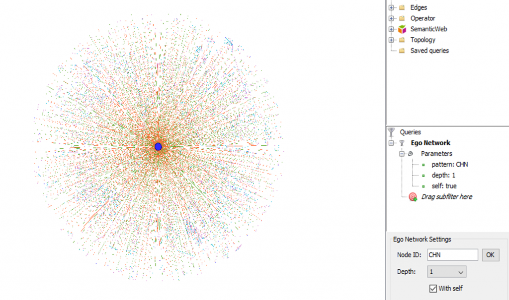
The goal of this exercise was to create team level graphs, which will each have a small subset of the entire dataset. One easy way to achieve this is to use the Ego Network filter to select a single team and its connections. Setting the ego network to a depth of 1 limits the display to only first degree connections; in this case players traded to or from our selected team.

Ego network with depth = 1

Once this step has been taken, we can then refine the display by applying another algorithm; in this case I have chosen the Yifan Hu option, and adjusted the settings until they created an aesthetically pleasing graph. The Yifan Hu adds further precision within each of the team graphs, and provides them with a common look & feel inasmuch as their respective data allows.

We have now completed our basic graph creation in Gephi, and can output our results to a variety of output formats. Our choice here is to create a GEXF file, which we can then plug in to an existing template. We do have another step with respect to the GEXF data. In order to relate the graphs back to their respective teams, I chose to apply official team colors to elements in the graph. Specifically, each node should reflect the individual team; we want the edges to remain the same across all graphs so that users have a common understanding for the types of connections between players and teams. So to update the node colors, simply use a code editor that can perform batch updates. I typically work with Brackets for this task, but choose your tool of choice. Here’s a view of the GEXF output prior to applying color changes:

GEXF nodes with original colors

Now here’s the updated version that reflects the Tigers navy blue coloring:

GEXF nodes updated with team colors

Once this step has been completed, I can upload the files to the web server, where other minor changes can be made. These include any updates to the CSS styling, adjustments to the config.js file, and minor changes to the index.html file so the proper team information is displayed. The easiest way to do this is to create a common set of directories for the basic javascript and CSS files, leaving only the individual config, html, and gexf files in each team’s directory.

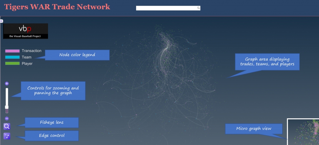
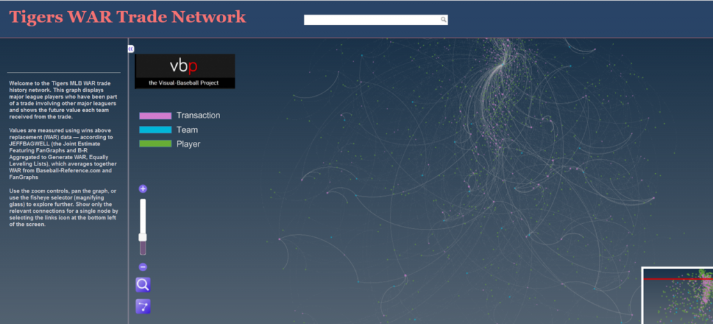
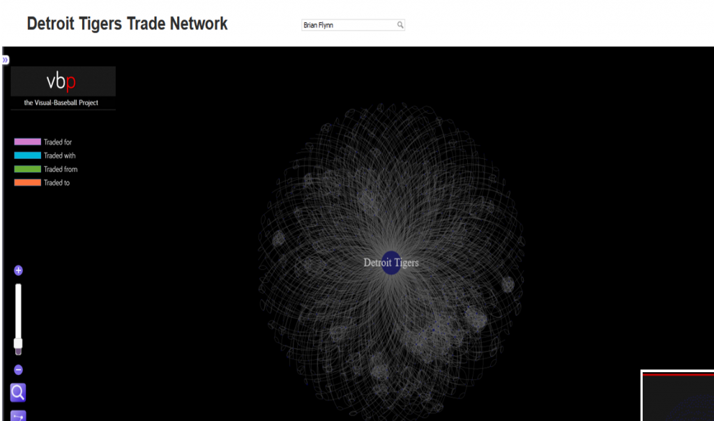
After a bit of massaging the config and CSS settings, the result is visually appealing as well as highly functional. Here’s a zoomed in look at the Toronto Blue Jays network on the web:

Blue Jays trade network close-up

All of the networks can be found by clicking the link below, with new ones being added until all teams have been represented:

Trade Networks

If you want to see each network in its own window or tab, use the right-click options in Firefox or Chrome.

I hope this has been helpful, and please feel free to reach out via the LinkedIn or Facebook Gephi groups, or leave a comment on this site.

Thanks for reading!

FacebooktwitterlinkedinrssFacebooktwitterlinkedinrssby feather
FacebooktwitterredditpinterestlinkedinmailFacebooktwitterredditpinterestlinkedinmailby feather

MLB Trades Network Map

Took a little break from the book to create a new infographic on trades between major league baseball teams over the last 100+ seasons, from 1901-2012. Network maps are often put to use analyzing and depicting connections within a social network like Twitter or Facebook, but can be used in many other instances, as this example shows.

The key concepts in network maps are nodes and edges; nodes are the connection points in a network (the teams in this case), while edges are the connections between nodes, showing a level of activity or connectedness (number of trades in this case). Have a look:

Network maps are often among the most elegant data visualizations, bordering on the artistic while still providing insight into the underlying data. In some cases, the maps are interactive, making them even more useful. At some point, I’ll offer some of those up, but in the meantime, take a look at the work of Jan-Willem Tulp and Jerome Cukier. These guys are creating some of the best work I’ve seen, highlighted by Tulp’s voting display from the 2012 Dutch elections, and Cukier’s interactive Paris Metro display. Fantastic work!

To view or download a PDF of the MLB trades graphic, click here.

FacebooktwitterlinkedinrssFacebooktwitterlinkedinrssby feather
FacebooktwitterredditpinterestlinkedinmailFacebooktwitterredditpinterestlinkedinmailby feather