Category: Player Networks

Updating Baseball Team Networks – Part 1

A few years back, I used Gephi and sigma.js to create a series of interactive baseball team networks, one for each current MLB franchise. These networks displayed all players through the 2013 season, going all the way back to 1901 for the original American and National League franchises. Now that we have data through the 2017 season, it’s time for an update, not only from a data perspective, but also stylistically. This post will walk through the process of creating one of these networks using Toad for MySQL, Gephi, and sigma.js to create web-based interactive network visualizations.

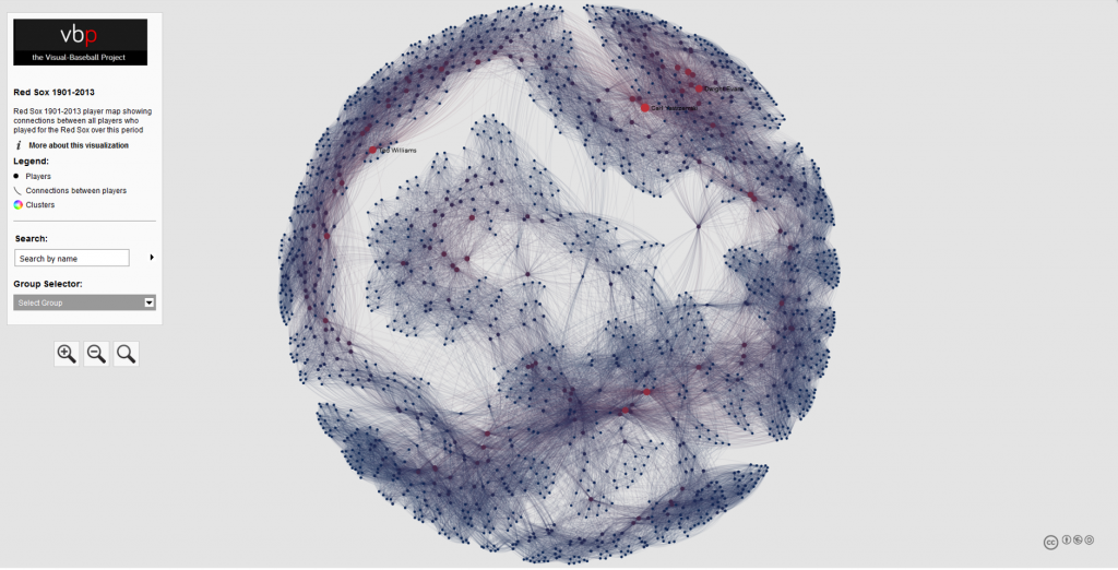
Here’s a typical network from the 2013 series; the full list of networks can be found here. We’ll use the existing networks as a baseline for the new networks, although a few modifications will be made.

baseball_team_network_2013
a 2013 baseball team network for the Boston Red Sox

Source Data & MySQL Queries

Let’s start our discussion with the source data. Season-level baseball data is available through the seanlahman.com website, in the form of .csv files or Microsoft Access database tables. I use the .csv format, as it can be easily added to existing MySQL databases on the visual-baseball.com server. MySQL also makes it simple to add derived fields through some simple coding. These fields can be utilized later for a variety of activities.

For the purpose of our network graphs, there are a handful of critical fields we want to use. These include the following:

  • playerID, a unique identifier for every player who ever donned a major league uniform
  • player name, which can be used to provide a meaningful reference based on the playerID field
  • yearID, which refers to the season (or seasons) a player suited up for a specific franchise
  • franchID, a unique identifier for each MLB franchise

We also need to do a little manipulation of the source data in our code to deliver our results in the proper form for use in Gephi. This means we need to create two input files – one for nodes, and a second for edges. The nodes will contain information about each player, the number of seasons played for the franchise and the first and last seasons, which may differ from the number of seasons, as players frequently leave a franchise only to return later in their career. Here’s our node code:

SELECT Id, Label, MAX(Size) as Size
FROM
(SELECT bp.playerID AS Id, CONCAT(bp.name, ” “, MIN(bp.yearID), “-“, MAX(bp.yearID)) AS Label, COUNT(bp.yearID) AS Size
FROM BattingPlus bp
WHERE bp.franchID = ‘BOS’ and bp.yearID >= 1901
GROUP BY bp.name

UNION ALL

SELECT pp.playerID AS Id, CONCAT(pp.name, ” “, MIN(pp.yearID), “-“, MAX(pp.yearID)) AS Label, COUNT(pp.yearID) AS Size
FROM BattingPlus pp
WHERE pp.franchID = ‘BOS’ and pp.yearID >= 1901
GROUP BY pp.name)  a
GROUP BY Id
ORDER BY Id;

Here’s the simple interpretation – since we are attempting to display all players for a given franchise, we are executing a UNION ALL statement to combine batters and pitchers into a single result file. We have used the playerID field to create the required Id value for Gephi, while also creating a Label field by combining the player’s name with their first and last years playing for this franchise. Finally, we have created a Size field based on the number of seasons played for the franchise. We can then choose to use this in Gephi to size each node, if we so choose.

We also need to create the edge file for Gephi. In this case, we want to understand how many seasons two players were on the same team. This code is a bit trickier, since we want to show only one connection between two players, since this will be an undirected graph. More on that distinction later. Here’s our edge code:

SELECT b.playerID AS Source, m.playerID  AS Target,  ‘Undirected’ as Type,  ‘ ‘ as Id, ‘ ‘ as Label, count(*) as weight
FROM
(SELECT a.playerID, CONCAT(m.nameFirst, ” “, m.nameLast) name, a.yearID, a.franchID

FROM Appearances a
INNER JOIN Master m
ON a.playerID = m.playerID

WHERE a.franchID = ‘BOS’ and a.yearID >= 1901) b

INNER JOIN Appearances a
ON b.yearID = a.yearID and b.franchID = a.franchID and b.playerID <> a.playerID and a.playerID > b.playerID
INNER JOIN Master m
ON a.playerID = m.playerID

GROUP BY b.playerID, a.playerID
ORDER BY b.playerID

Here we use the Master table to provide player name information, and we also gather the ID information to match the node values. The critical piece in this code is in our join criteria:

INNER JOIN Appearances a
ON b.yearID = a.yearID and b.franchID = a.franchID and b.playerID <> a.playerID and a.playerID > b.playerID

Here we are matching players based on the same season and the same franchise. We then specify that we do not want to connect any player to himself, and that we want only values where the playerID value from our main query is greater than the playerID value from the sub-query. This gives us a single connection between two players, which is what we need for an undirected graph. We then define a Source node (required by Gephi) and a Target node (also required), as well as specifying ‘Undirected’ as the graph type. We leave the ID and Label values empty, and then summarize the number of seasons played together as an edge weight. This value can be used in Gephi to show the strength of a connection between two nodes (e.g.- did they spend one season together, or 10 seasons together?).

After exporting each of these files to a .csv format, we have our source data for Gephi. In Part 2 our focus will shift to creating the network in Gephi.

Player Ego Network Visualization

Ego networks are an interesting concept within the realm of network visualization using graph analysis, as they allow us to easily see direct connections within the network of a particular individual. Using Gephi, we can navigate large networks using this technique, which enables us to filter and view only those connections relevant to our current criteria. All remaining nodes and edges are simply filtered out from a visual perspective, giving a very clean look at individual networks. The ego network can be set to a depth of 1 if the goal is to show only direct connections, or to 2 or even 3 if our goal is to see the so-called “friends of friends” via indirect connections.

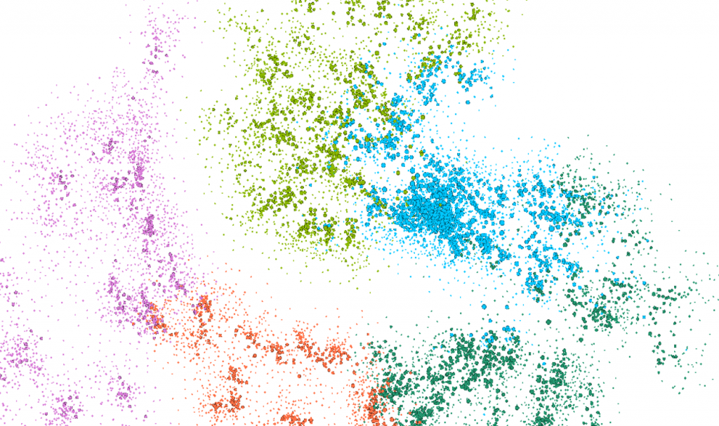
My latest venture uses a network of all MLB players between 1901 and 2015, which consists of a somewhat unwieldy mass of nearly 17,000 players with close to 1.2 million connections. Even when we cluster the results using Gephi’s modularity class option, it is still a difficult network to navigate, both from a visual perspective and a resource allocation viewpoint. Here’s a view of the network as a whole:

mlb_players_20161230

While the modularity class coloring helps identify groups of related players, there is an awful lot of small detail that is not easily discerned, and the graph is computationally expensive, often crashing my version of Gephi if I try to do too many things with the full graph. Fortunately, ego networks are a great way to filter the data for greater understanding of some of the details within the network.

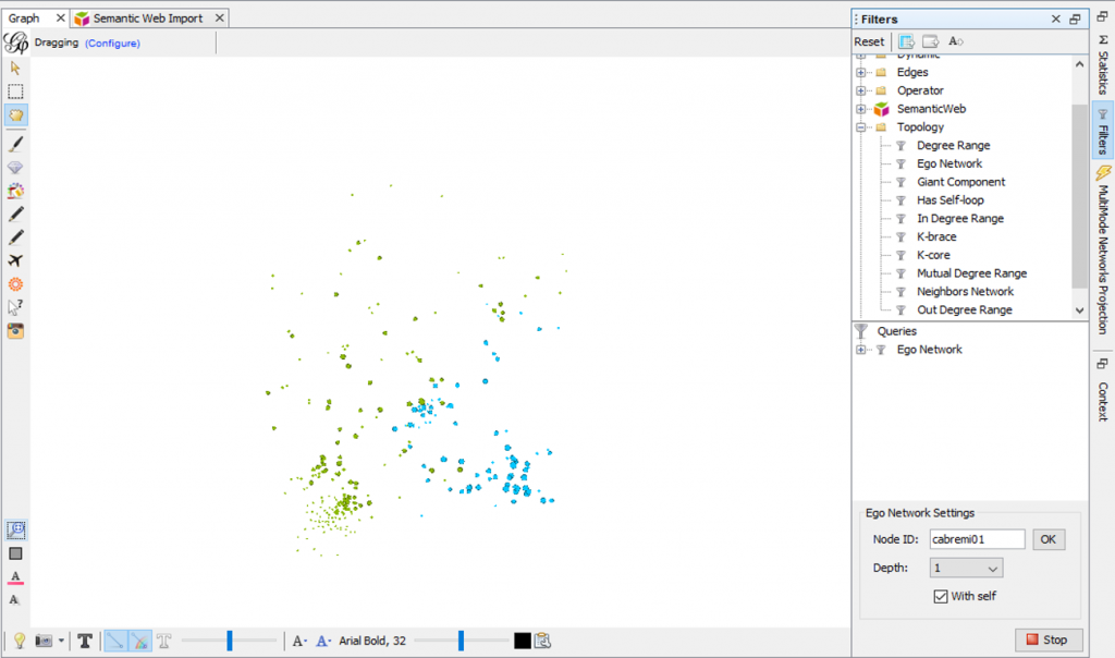
Using the ego network option as a filter, I am able to view the individual network of any player in the graph with ease. Here’s a look at my settings for the Miguel Cabrera ego network, and the resulting network, which is now a very manageable 300 nodes and 11k edges:

mlb_ego_filter_20161230

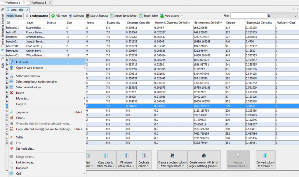
With a little editing in Gephi, such as increasing the size and adjusting the color for the central node, I can easily create a series of ego networks that can later be exported to a JSON format for use with Sigma.js. These can then be turned into interactive web-based networks quite easily. Here, we change the existing node settings so that the Cabrera node stands out in the graph. First, we locate Cabrera’s record in the data worksheet, and then select the node edit menu option:

mlb_edit_node1_20161230

This then takes us to the node properties, where size and color can be edited:

mlb_edit_node2_20161230

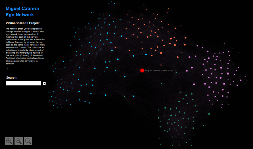
If this step causes some overlap in the graph, we can easily run the Noverlap layout algorithm to optimize graph spacing. Here’s a view of the completed Cabrera network after using Sigma.js and tweaking a few of the config settings:

Cabrera_20161130

As of now, there are five of these ego networks available for viewing on the visual-baseball site. They can be found here. I promise more to come in 2017 as time permits. Update – 25 networks as of 1/15/2017.

A Network Graph of MLB All-Stars

With the Major League Baseball All-Star game this week, I was suddenly possessed by an urge to create a network graph of all the players who have been selected for the game from 1933-2015. The goal, as with most of my network graph efforts, was to see where the data took me, and what stories it might tell. Along for the ride was my trusty companion Gephi, version 0.9.1 in this instance. Data for this exercise comes, as it so often does, from the Lahman baseball database, which happens to have a nice table with all the necessary all-star information.

The challenge inherent in this data, as with many temporal datasets, is to create an interesting graph that isn’t entirely driven by the time element, in this case as baseball seasons. Some otherwise excellent layout algorithms tend to turn this sort of data into long, worm-like displays that are not visually appealing. I could just as easily use a timeline if that were the goal of the visualization. So in an effort to balance aesthetics with the underlying data, I finally settled on the radial axis layout in Gephi. With this layout, we have the ability to create multiple axes radiating from the center of the graph, grouped by something meaningful. In this case, that turns out to be the modularity class, a sort of clustering mechanism that groups nodes together based on common or similar characteristics.

After some trial and error, I wound up with 13 distinct classes, a nice manageable number for this type of display. The end result can be interpreted as some sort of exotic, colorful starfish, or perhaps as a multi-colored fireworks display. In any event, I believe it tells an interesting story in a visually appealing manner, and allows for understanding the common threads within each cluster of players. Here’s the complete graph layout:

allstar_graph_base

I’ll spend the rest of the post with some quick analyses of each group, and then point you to the entire graph in interactive form so you can discover your own patterns and learn more about the all-star connections of individual players. I’ll also provide a quick overview for how to read the sidebar output for the graph when you interact with the data.

Our 13 clusters (you can think of them as cohorts) tell us some interesting things about the history of all-star participants. Let’s walk through each of the 13 (numbered 0 through 12) to learn more. The clusters begin with 0 (in green) at the upper left and move counter-clockwise around the graph. Each is rank ordered from small to large radiating out from the center, so the member with the most years as an all-star will be at the tip of each group. That individual will serve as our focal point in each of the following screenshots, followed by a brief overview of other members of the cohort.

First up is our Cohort 0, headlined by Miguel Cabrera, with 10 selections through 2015. Obviously, this would appear to be a cohort of current or recent all-stars based on Cabrera’s appearance. We can easily navigate the graph to see if that’s the case. Who else is prominent in the group? Yadier Molina, Matt Holliday, and Robinson Cano, to name a few, all big name stars for most of their careers. How about at the low end of the spectrum, players with a single all-star selection? Here’s where we find the likes of Billy Butler, R.A. Dickey, and Melky Cabrera. All long-tenured, noteworthy players, but certainly not in the same category as the first group.

cohort_0

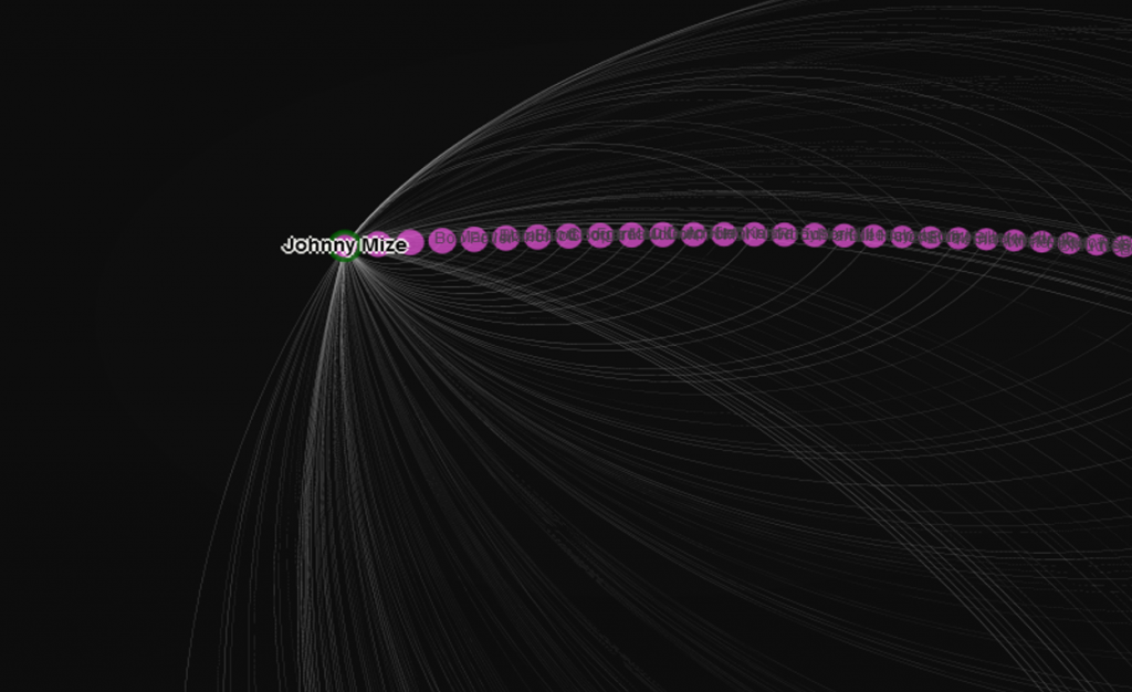
Cohort 1 takes us on some time travel, with Johnny Mize as the representative star, also with 10 all-star selections and Hall of Fame membership as well. Joining Mize in the group are Bobby Doerr, Vern Stephens, Joe Gordon, and Bob Feller, all Hall of Famers with the exception of Stephens. At the other end of the cohort, each with one appearance, are Oscar Grimes, Red Barrett, and Nick Etten, among others. Based on the career arcs of the stars in this group, we could characterize it as primarily a 1940s-based cohort, certainly with overlap into the surrounding decades.

cohort_1

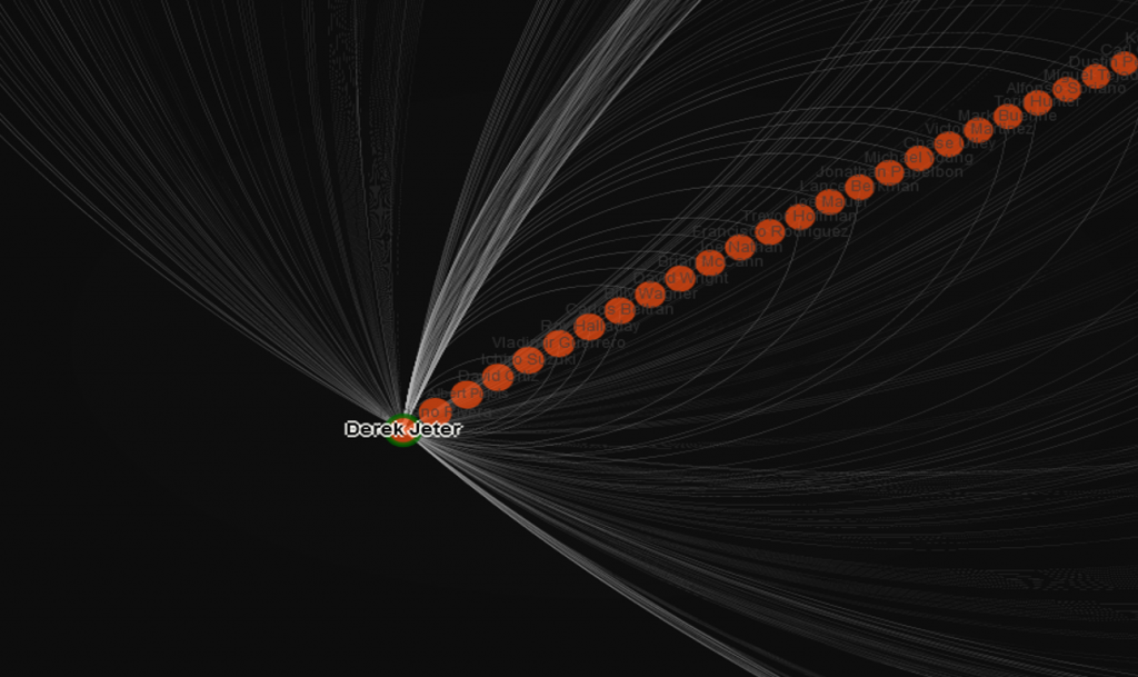
Derek Jeter is our icon for Cohort 2, so it figures to be a group that immediately precedes the Cabrera-led Cohort 0. Perhaps the focus here will be on stars from the early 2000s, at the center point of Jeter’s long career. Mariano Rivera, Albert Pujols, and David Ortiz are among the top stars here, confirming the hypothesis that this group is largely post-2000 in nature. Among the lesser knowns with a single selection each are Gil Meche, Joe Crede, and Ryan Ludwick.

cohort_2

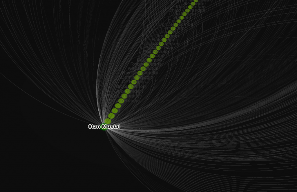
Cohort 3 is headed up by the legendary Stan Musial, whose career covered the entirety of the 40s and 50s. Given that Cohort 1 was largely concentrated on players from the 40s, we might anticipate more of a skew towards 1950 and beyond. We’ll see in a moment if that’s true. Next to Musial we have Ted Williams and Warren Spahn, two more whose careers spanned both decades, so perhaps we have players here with greater longevity compared to the Mize cohort. Let’s go a bit deeper, where we find Roy Campanella, Larry Doby, and Robin Roberts, all with career pinnacles primarily in the 50s. So while there will certainly be connections across the two groups, Cohort 3 does appear to span more of the 1950s compared to Cohort 1.

cohort_3

With Cohort 4 we see a very large group fronted by all-time hits leader Pete Rose. So we could be focused on the 1960s or 1970s here; Rod Carew, Reggie Jackson, and Mike Schmidt, Hall of Famers all, are included, so the 1970s would seem to be the dominant theme. Perhaps we shouldn’t be surprised at the size of this group, as expansion in the 1960s afforded more players the opportunity to become an all-star. A few interesting figures can be found at the single game end of the radian – Bob Horner, Kent Hrbek, and Lonnie Smith, all with at least momentary brushes with greatness, but good enough to qualify for just one all-star nod apiece.

cohort_4

Joe DiMaggio is the lead for our next group, joined by the likes of Mel Ott, Bill Dickey, and Joe Medwick. The skew is toward the late 1930s and beyond; many members of this cohort would have had limited all-star game opportunities, as the game originated only in 1933. As proof of this, we find Hall of Famers Heinie Manush, Goose Goslin, and Kiki Cuyler at the low end of the radian, each with just a single all-star credit.

cohort_5

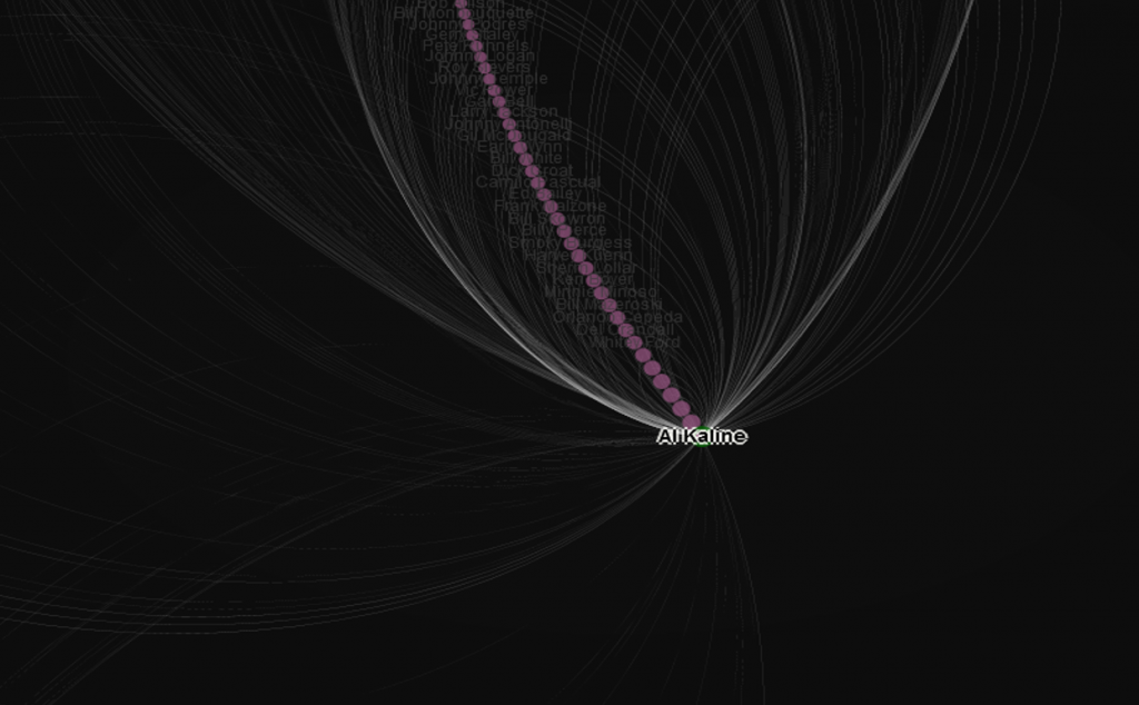
Hall of Famer Al Kaline heads up Cohort 6, so we know we’re in either the 50s or 60s, or more likely, a bit of both decades. Along with Kaline we have Mickey Mantle, Yogi Berra, and Ernie Banks, each of who had multiple appearances covering both decades. At the more modest end of the group we find Rocky Bridges, Bob Cerv, and perhaps surprisingly, the slugger Joe Adcock, each with just a single season as all-stars.

cohort_6

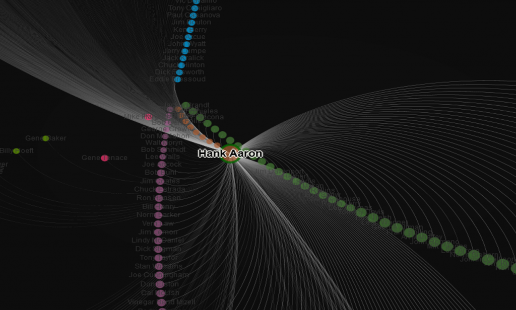
Cohort 7 is our one group that’s difficult to explain. Our graph modularity settings forced a small cohort of just nine players; Hank Aaron with 21 seasons, and eight others with a single season each. Consider this one a bit of a fluke.

cohort_7

The great Willie Mays leads the relatively small Cohort 8, joined by both Brooks and Frank Robinson, as well as Roberto Clemente. This would indicate a cohort of players who began in the 1950s and perhaps peaked in the 60s. Lower down the list this group features lesser known players like Tito Francona, Dick Howser, and Joey Jay, all one season all-stars.

cohort_8

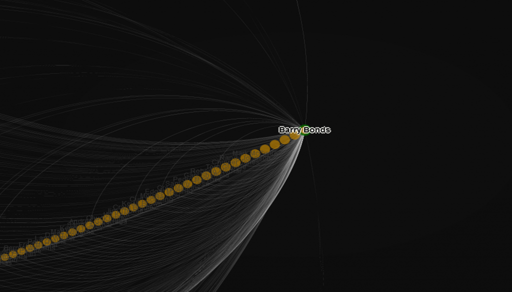
Cohort 9 is a very large group led by Barry Bonds, Ivan “Pudge” Rodriguez, and Ken Griffey. Here we have three stars with illustrious careers launched around 1990 and extending into the new millenium. At the other extreme we find one-timers such as Jay Buhner, Mark Grudzelianek, and Lance Johnson.

cohort_9

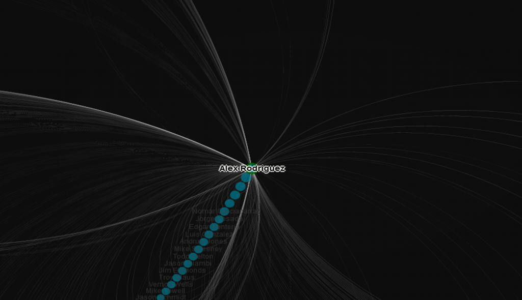
Cohort 10 is a mid-sized group headed up by Alex Rodriguez, and featuring Manny Ramirez, John Smoltz, and Scott Rolen. This would appear to be a very similar group (if a few years later) to the prior cohort, and we should expect to find a great number of crossover connections between the two, as they each cover players from similar time periods.

cohort_10

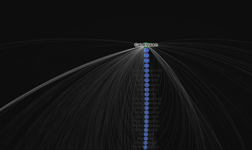
Down to the final two groups! Cohort 11 is led by Cal Ripken, Ozzie Smith, and Roger Clemens, all major impact players in both the 1980s and 90s. This is another group featuring players who were quite talented but dented the all-star ranks just a single time. Among these were outfielders Jesse Barfield and Kevin Bass, and pitcher Teddy Higuera.

cohort_11

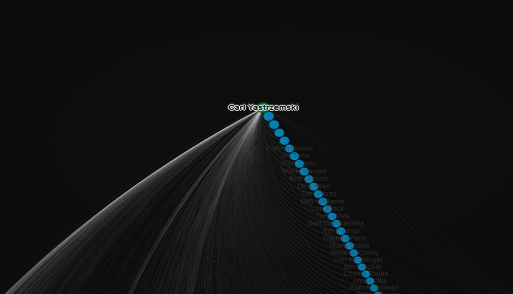
With Cohort 12, we see a large group led by 18-time all-star Carl Yastrzemski, supported by Johnny Bench, Tom Seaver, and Harmon Killebrew. These are all players who were at their productive peaks in the late 1960s through mid-1970s, an era where the National League was dominating the annual game. Chuck Hinton, Jerry Lumpe, and Joe Azcue are among those who can claim a single trip to the all-star game as a career highlight.

cohort_12

Quick note on the sidebar – you’ll see a few measures which I won’t go into too deeply here; there are 3 centrality measures (influence within the network), eccentricity (the number of steps to traverse the network, think six degrees of Kevin Bacon), and size, reflecting the number of seasons as an all-star. The key part of the sidebar lies in the listing of all connected players to the one currently selected, with numbers indicating the number of games as co-all-stars. Use these links to navigate through the network quickly. It’s fun!

So that’s it for our brief analysis. Now it’s time to explore for yourself by opening the MLB All-Star Network visualization. Be patient as the data loads; once it has cached the graph should be fairly fast at zooming, panning, and allowing you to explore to your heart’s content.